Python NumPy 入门教程

本文是 Python 科学计算库numpy、scipy及matplotlib的快速入门教程，翻译自斯坦福大学 CS231n - Python NumPy Tutorial 。

NumPy

NumPy是Python中科学计算的核心库。它提供了一个高性能的多维数组对象，以及使用这些数组的工具。

数组

NumPy的核心功能是"ndarray"（即n-dimensional array，多维数组） 数据结构。这是一个表示多维度、同质并且固定大小的数组对象。维数是数组的秩 rank ; 数组的形状 shape 是一个整数元组，表示沿着每个维度的数组大小。

我们可以从嵌套的Python列表初始化numpy数组，并使用方括号来访问元素：

import numpy as np

a = np.array([1, 2, 3])  # Create a rank 1 array
print type(a)            # Prints "<type 'numpy.ndarray'>"
print a.shape            # Prints "(3,)"
print a[0], a[1], a[2]   # Prints "1 2 3"
a[0] = 5                 # Change an element of the array
print a                  # Prints "[5, 2, 3]"

b = np.array([[1,2,3],[4,5,6]])   # Create a rank 2 array
print b.shape                     # Prints "(2, 3)"
print b[0, 0], b[0, 1], b[1, 0]   # Prints "1 2 4"

NumPy还提供许多创建数组的函数：

import numpy as np

a = np.zeros((2,2))  # Create an array of all zeros
print a              # Prints "[[ 0.  0.]
                     #          [ 0.  0.]]"
    
b = np.ones((1,2))   # Create an array of all ones
print b              # Prints "[[ 1.  1.]]"

c = np.full((2,2), 7) # Create a constant array
print c               # Prints "[[ 7.  7.]
                      #          [ 7.  7.]]"

d = np.eye(2)        # Create a 2x2 identity matrix
print d              # Prints "[[ 1.  0.]
                     #          [ 0.  1.]]"
    
e = np.random.random((2,2)) # Create an array filled with random values
print e                     # Might print "[[ 0.91940167  0.08143941]
                            #               [ 0.68744134  0.87236687]]"

你可以在 这份文档 中阅读关于数组创建的其他方法。

数组索引

NumPy提供了多种索引到数组的方法。

切片：与Python列表类似，可以对numpy数组进行切片。由于数组可能是多维的，因此必须为数组的每个维度指定一个切片：

import numpy as np

# Create the following rank 2 array with shape (3, 4)
# [[ 1  2  3  4]
#  [ 5  6  7  8]
#  [ 9 10 11 12]]
a = np.array([[1,2,3,4], [5,6,7,8], [9,10,11,12]])

# Use slicing to pull out the subarray consisting of the first 2 rows
# and columns 1 and 2; b is the following array of shape (2, 2):
# [[2 3]
#  [6 7]]
b = a[:2, 1:3]

# A slice of an array is a view into the same data, so modifying it
# will modify the original array.
print a[0, 1]   # Prints "2"
b[0, 0] = 77    # b[0, 0] is the same piece of data as a[0, 1]
print a[0, 1]   # Prints "77"

你还可以将整数索引与片段索引进行混合。但是，这样做会产生比原始数组更低的数组：

import numpy as np

# Create the following rank 2 array with shape (3, 4)
# [[ 1  2  3  4]
#  [ 5  6  7  8]
#  [ 9 10 11 12]]
a = np.array([[1,2,3,4], [5,6,7,8], [9,10,11,12]])

# Two ways of accessing the data in the middle row of the array.
# Mixing integer indexing with slices yields an array of lower rank,
# while using only slices yields an array of the same rank as the
# original array:
row_r1 = a[1, :]    # Rank 1 view of the second row of a  
row_r2 = a[1:2, :]  # Rank 2 view of the second row of a
print row_r1, row_r1.shape  # Prints "[5 6 7 8] (4,)"
print row_r2, row_r2.shape  # Prints "[[5 6 7 8]] (1, 4)"

# We can make the same distinction when accessing columns of an array:
col_r1 = a[:, 1]
col_r2 = a[:, 1:2]
print col_r1, col_r1.shape  # Prints "[ 2  6 10] (3,)"
print col_r2, col_r2.shape  # Prints "[[ 2]
                            #          [ 6]
                            #          [10]] (3, 1)"

整数数组索引：当你使用切片索引到numpy数组时，生成的数组视图将始终是原始数组的子数组。 相反，整数数组索引允许你使用另一个数组的数据来构造任意数组。 例如：

import numpy as np

a = np.array([[1,2], [3, 4], [5, 6]])

# An example of integer array indexing.
# The returned array will have shape (3,) and 
print a[[0, 1, 2], [0, 1, 0]]  # Prints "[1 4 5]"

# The above example of integer array indexing is equivalent to this:
print np.array([a[0, 0], a[1, 1], a[2, 0]])  # Prints "[1 4 5]"

# When using integer array indexing, you can reuse the same
# element from the source array:
print a[[0, 0], [1, 1]]  # Prints "[2 2]"

# Equivalent to the previous integer array indexing example
print np.array([a[0, 1], a[0, 1]])  # Prints "[2 2]"

一个有用的整数数组索引技巧，是从矩阵的每一行中选择一个元素：

import numpy as np

# Create a new array from which we will select elements
a = np.array([[1,2,3], [4,5,6], [7,8,9], [10, 11, 12]])

print a  # prints "array([[ 1,  2,  3],
         #                [ 4,  5,  6],
         #                [ 7,  8,  9],
         #                [10, 11, 12]])"

# Create an array of indices
b = np.array([0, 2, 0, 1])

# Select one element from each row of a using the indices in b
print a[np.arange(4), b]  # Prints "[ 1  6  7 11]"

# Mutate one element from each row of a using the indices in b
a[np.arange(4), b] += 10

print a  # prints "array([[11,  2,  3],
         #                [ 4,  5, 16],
         #                [17,  8,  9],
         #                [10, 21, 12]])

布尔数组索引：布尔数组索引可以让你选择数组的任意元素。通常，这种类型的索引用于选择满足某些条件的数组的元素。例如：

import numpy as np

a = np.array([[1,2], [3, 4], [5, 6]])

bool_idx = (a > 2)  # Find the elements of a that are bigger than 2;
                    # this returns a numpy array of Booleans of the same
                    # shape as a, where each slot of bool_idx tells
                    # whether that element of a is > 2.
            
print bool_idx      # Prints "[[False False]
                    #          [ True  True]
                    #          [ True  True]]"

# We use boolean array indexing to construct a rank 1 array
# consisting of the elements of a corresponding to the True values
# of bool_idx
print a[bool_idx]  # Prints "[3 4 5 6]"

# We can do all of the above in a single concise statement:
print a[a > 2]     # Prints "[3 4 5 6]"

为了简洁起见，我们省略了很多有关numpy数组索引的细节；如果你想了解更多，请阅读 这份文档 。

数组计算

基本的数学函数在数组上按元素运算，并且可以作为运算符重载和numpy模块中的函数使用：

import numpy as np

x = np.array([[1,2],[3,4]], dtype=np.float64)
y = np.array([[5,6],[7,8]], dtype=np.float64)

# Elementwise sum; both produce the array
# [[ 6.0  8.0]
#  [10.0 12.0]]
print x + y
print np.add(x, y)

# Elementwise difference; both produce the array
# [[-4.0 -4.0]
#  [-4.0 -4.0]]
print x - y
print np.subtract(x, y)

# Elementwise product; both produce the array
# [[ 5.0 12.0]
#  [21.0 32.0]]
print x * y
print np.multiply(x, y)

# Elementwise division; both produce the array
# [[ 0.2         0.33333333]
#  [ 0.42857143  0.5       ]]
print x / y
print np.divide(x, y)

# Elementwise square root; produces the array
# [[ 1.          1.41421356]
#  [ 1.73205081  2.        ]]
print np.sqrt(x)

请注意，*是元素乘法，而不是矩阵乘法。如需使用矩阵乘法，请使用函数dot。dot可用作numpy模块中的函数，也可用作数组对象的实例方法：

import numpy as np

x = np.array([[1,2],[3,4]])
y = np.array([[5,6],[7,8]])

v = np.array([9,10])
w = np.array([11, 12])

# Inner product of vectors; both produce 219
print v.dot(w)
print np.dot(v, w)

# Matrix / vector product; both produce the rank 1 array [29 67]
print x.dot(v)
print np.dot(x, v)

# Matrix / matrix product; both produce the rank 2 array
# [[19 22]
#  [43 50]]
print x.dot(y)
print np.dot(x, y)

NumPy提供了许多有用的矩阵计算函数；其中最重要的函数之一是sum：

import numpy as np

x = np.array([[1,2],[3,4]])

print np.sum(x)  # Compute sum of all elements; prints "10"
print np.sum(x, axis=0)  # Compute sum of each column; prints "[4 6]"
print np.sum(x, axis=1)  # Compute sum of each row; prints "[3 7]"

你可以在 这份文档 中找到numpy提供的数学函数完整列表。

除了使用数组计算数学函数之外，我们经常需要重新整形或以其他方式处理数组中的数据。 这种类型的操作的最简单的例子是转置矩阵；要转置矩阵，只需使用数组对象的T属性：

import numpy as np

x = np.array([[1,2], [3,4]])
print x    # Prints "[[1 2]
           #          [3 4]]"
print x.T  # Prints "[[1 3]
           #          [2 4]]"

# Note that taking the transpose of a rank 1 array does nothing:
v = np.array([1,2,3])
print v    # Prints "[1 2 3]"
print v.T  # Prints "[1 2 3]"

NumPy提供了更多的功能来操作数组；你可以在 这份文档 中看到完整列表。

广播

广播是一种强大的机制，允许numpy在执行算术运算时使用不同形状的数组。 通常我们有一个更小的数组和一个更大的数组，我们想要使用较小的数组多次来对较大的数组执行一些操作。

例如，假设我们要为矩阵的每一行添加一个常量向量。 我们可以这样做：

import numpy as np

# We will add the vector v to each row of the matrix x,
# storing the result in the matrix y
x = np.array([[1,2,3], [4,5,6], [7,8,9], [10, 11, 12]])
v = np.array([1, 0, 1])
y = np.empty_like(x)   # Create an empty matrix with the same shape as x

# Add the vector v to each row of the matrix x with an explicit loop
for i in range(4):
    y[i, :] = x[i, :] + v

# Now y is the following
# [[ 2  2  4]
#  [ 5  5  7]
#  [ 8  8 10]
#  [11 11 13]]
print y

这种方法是可以的；然而，当矩阵x非常大时，Python循环可能会运行很长时间。实际上，将向量v添加到矩阵x的每一行，等价于通过创建垂直堆叠v的矩阵vv，然后执行x和vv的元素求和。我们可以这样实现这个方法：

import numpy as np

# We will add the vector v to each row of the matrix x,
# storing the result in the matrix y
x = np.array([[1,2,3], [4,5,6], [7,8,9], [10, 11, 12]])
v = np.array([1, 0, 1])
vv = np.tile(v, (4, 1))  # Stack 4 copies of v on top of each other
print vv                 # Prints "[[1 0 1]
                         #          [1 0 1]
                         #          [1 0 1]
                         #          [1 0 1]]"
y = x + vv  # Add x and vv elementwise
print y  # Prints "[[ 2  2  4
         #          [ 5  5  7]
         #          [ 8  8 10]
         #          [11 11 13]]"

NumPy的广播允许我们在不创建v的多个副本的情况下执行这个计算。以上情况下，我们可以使用广播：

import numpy as np

# We will add the vector v to each row of the matrix x,
# storing the result in the matrix y
x = np.array([[1,2,3], [4,5,6], [7,8,9], [10, 11, 12]])
v = np.array([1, 0, 1])
y = x + v  # Add v to each row of x using broadcasting
print y  # Prints "[[ 2  2  4]
         #          [ 5  5  7]
         #          [ 8  8 10]
         #          [11 11 13]]"

即使 x具有形状 (4, 3) 且v具有形状 (3,)，行y = x + v可以正常执行；工作原理是由于广播，v仿佛有形状(4, 3) ，其中每行都是v的副本，然后以按元素方式进行求和。

两个数组间的广播遵循以下规则：

1. 如果阵列不具有相同的秩，则对较小秩的阵列进行预处理，直到两个形状都具有相同的长度。
2. 如果两个数组在某一维度的大小相等，或者其中一个数组在该维度的大小为1，则称两个数组在这个维度上兼容。
3. 如果两个数组在所有维度上都兼容，则可以进行广播。
4. 广播后，每个数组形状等同于较大的数组形状。
5. 如果在某一维度，其中一个数组大小等于1并且另一个数组大小大于1，则前者沿着此维度复制自身。

如果感到困惑，请尝试阅读 这份文档 或 这份说明 。

支持广播的函数被称为通用函数。你可以在 这份文档 中找到所有通用函数的列表。 以下是广播的一些应用：

import numpy as np

# Compute outer product of vectors
v = np.array([1,2,3])  # v has shape (3,)
w = np.array([4,5])    # w has shape (2,)
# To compute an outer product, we first reshape v to be a column
# vector of shape (3, 1); we can then broadcast it against w to yield
# an output of shape (3, 2), which is the outer product of v and w:
# [[ 4  5]
#  [ 8 10]
#  [12 15]]
print np.reshape(v, (3, 1)) * w

# Add a vector to each row of a matrix
x = np.array([[1,2,3], [4,5,6]])
# x has shape (2, 3) and v has shape (3,) so they broadcast to (2, 3),
# giving the following matrix:
# [[2 4 6]
#  [5 7 9]]
print x + v

# Add a vector to each column of a matrix
# x has shape (2, 3) and w has shape (2,).
# If we transpose x then it has shape (3, 2) and can be broadcast
# against w to yield a result of shape (3, 2); transposing this result
# yields the final result of shape (2, 3) which is the matrix x with
# the vector w added to each column. Gives the following matrix:
# [[ 5  6  7]
#  [ 9 10 11]]
print (x.T + w).T
# Another solution is to reshape w to be a column vector of shape (2, 1);
# we can then broadcast it directly against x to produce the same
# output.
print x + np.reshape(w, (2, 1))

# Multiply a matrix by a constant:
# x has shape (2, 3). NumPy treats scalars as arrays of shape ();
# these can be broadcast together to shape (2, 3), producing the
# following array:
# [[ 2  4  6]
#  [ 8 10 12]]
print x * 2

广播通常会使你的代码更加简洁快捷，因此你应尽可能地努力使用它。

NumPy文档

这个简短的概述已经涉及到大部分numpy的重要功能，但仍有许多地方未涉及。查看 numpy参考文档 以了解更多关于numpy的信息。

SciPy

NumPy提供了一个高性能的多维数组和基本的工具来计算和操纵这些数组。 SciPy建立在此基础之上，并提供了大量功能，可以运行在numpy数组上，并且可用于不同类型的科学和工程应用。

熟悉SciPy的最佳方法是浏览 这份文档 。我们将阐述SciPy的一些对神经网络有用的部分。

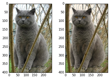
图像操作

SciPy提供了一些基本功能来处理图像。例如，它具有从磁盘读取图像到numpy数组，将numpy数组写入磁盘作为图像并调整图像大小的功能。下面的示例中展示了这些功能：

from scipy.misc import imread, imsave, imresize

# Read an JPEG image into a numpy array
img = imread('assets/cat.jpg')
print img.dtype, img.shape  # Prints "uint8 (400, 248, 3)"

# We can tint the image by scaling each of the color channels
# by a different scalar constant. The image has shape (400, 248, 3);
# we multiply it by the array [1, 0.95, 0.9] of shape (3,);
# numpy broadcasting means that this leaves the red channel unchanged,
# and multiplies the green and blue channels by 0.95 and 0.9
# respectively.
img_tinted = img * [1, 0.95, 0.9]

# Resize the tinted image to be 300 by 300 pixels.
img_tinted = imresize(img_tinted, (300, 300))

# Write the tinted image back to disk
imsave('assets/cat_tinted.jpg', img_tinted)

---

---

点的距离

SciPy定义了一些有用的函数，用于计算点集合之间的距离。

函数scipy.spatial.distance.pdist计算给定单个集合中所有点之间的距离：

import numpy as np
from scipy.spatial.distance import pdist, squareform

# Create the following array where each row is a point in 2D space:
# [[0 1]
#  [1 0]
#  [2 0]]
x = np.array([[0, 1], [1, 0], [2, 0]])
print x

# Compute the Euclidean distance between all rows of x.
# d[i, j] is the Euclidean distance between x[i, :] and x[j, :],
# and d is the following array:
# [[ 0.          1.41421356  2.23606798]
#  [ 1.41421356  0.          1.        ]
#  [ 2.23606798  1.          0.        ]]
d = squareform(pdist(x, 'euclidean'))
print d

你可以在 这份文档 中阅读有关此功能的所有详细信息。

类似的函数（scipy.spatial.distance.cdist）能够计算不同集合内所有点之间的距离；你可以阅读 这份文档 。

Matplotlib

Matplotlib 是一个绘图库。本节简要介绍了matplotlib.pyplot模块，该模块提供了与MATLAB类似的绘图系统。

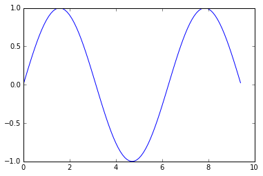
绘图

matplotlib中最重要的函数是plot，它可以绘制2D数据。这是一个简单的例子：

import numpy as np
import matplotlib.pyplot as plt

# Compute the x and y coordinates for points on a sine curve
x = np.arange(0, 3 * np.pi, 0.1)
y = np.sin(x)

# Plot the points using matplotlib
plt.plot(x, y)
plt.show()  # You must call plt.show() to make graphics appear.

运行此代码，会生成以下图形：

---

---

只需一点额外的工作，我们可以轻松地绘制多行，并添加标题，图例和轴标签：

import numpy as np
import matplotlib.pyplot as plt

# Compute the x and y coordinates for points on sine and cosine curves
x = np.arange(0, 3 * np.pi, 0.1)
y_sin = np.sin(x)
y_cos = np.cos(x)

# Plot the points using matplotlib
plt.plot(x, y_sin)
plt.plot(x, y_cos)
plt.xlabel('x axis label')
plt.ylabel('y axis label')
plt.title('Sine and Cosine')
plt.legend(['Sine', 'Cosine'])
plt.show()

---

---

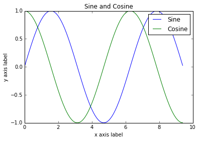
关于plot函数的更多信息，你可以阅读 这份文档 。

绘制子图

你可以使用subplot函数在同一图中绘制不同子图。例如：

import numpy as np
import matplotlib.pyplot as plt

# Compute the x and y coordinates for points on sine and cosine curves
x = np.arange(0, 3 * np.pi, 0.1)
y_sin = np.sin(x)
y_cos = np.cos(x)

# Set up a subplot grid that has height 2 and width 1,
# and set the first such subplot as active.
plt.subplot(2, 1, 1)

# Make the first plot
plt.plot(x, y_sin)
plt.title('Sine')

# Set the second subplot as active, and make the second plot.
plt.subplot(2, 1, 2)
plt.plot(x, y_cos)
plt.title('Cosine')

# Show the figure.
plt.show()

---

---

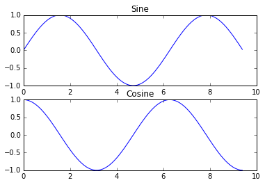
关于subplot函数的更多信息，你可以阅读 这份文档 。

图片

你可以使用imshow功能来显示图像。例如：

import numpy as np
from scipy.misc import imread, imresize
import matplotlib.pyplot as plt

img = imread('assets/cat.jpg')
img_tinted = img * [1, 0.95, 0.9]

# Show the original image
plt.subplot(1, 2, 1)
plt.imshow(img)

# Show the tinted image
plt.subplot(1, 2, 2)

# A slight gotcha with imshow is that it might give strange results
# if presented with data that is not uint8. To work around this, we
# explicitly cast the image to uint8 before displaying it.
plt.imshow(np.uint8(img_tinted))
plt.show()

---

---