本文翻译自 TensorFlow - Get Started 官方入门教程。
张量
TensorFlow 的核心单元是 张量(tensor)。张量是一个多维数组,其维度称为 秩(rank)。以下是张量的一些例子:
1 | 3 # a rank 0 tensor; this is a scalar with shape [] |
TensorFlow Core 教程
导入 TensorFlow
TensorFlow 的规范 import 语句如下:
1 | import tensorflow as tf |
这使的 Python 访问所有 TensorFlow 的类,方法和符号。
计算图
TensorFlow 核心方案为由两个独立的部分组成:
- 构建计算图。
- 运行计算图。
计算图是一系列对节点图的 TensorFlow 操作。下面建立一个简单的计算图表,每个节点输入零个或多个张量,并输出一个张量。节点的一种类型是常量 constant,不需要输入,输出为内部存储的值。创建两个浮点张量 node1 和 node2 如下:
1 | node1 = tf.constant(3.0, tf.float32) |
最后的 print 打印如下:
1 | Tensor("Const:0", shape=(), dtype=float32) Tensor("Const_1:0", shape=(), dtype=float32) |
请注意,节点的打印语句并不会输出节点的值 3.0 和 4.0 。要计算并输出节点的值,必须运行计算图的会话(Session)。会话封装了 TensorFlow 运行时的控制和状态。
以下代码创建一个 Session 对象,然后调用其 run 方法来通过计算图来得到 node1 和 node2 的值。在会话中运行计算图,结果如下:
1 | sess = tf.Session() |
输出结果为期望输出 3.0 和 4.0 :
1 | [3.0, 4.0] |
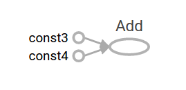
我们可以通过组合张量的节点与操作(操作也属于节点)来实现更复杂的计算。例如,我们可以添加我们的两个常量节点并生成一个新的图,如下所示:
1 | node3 = tf.add(node1, node2) |
最后两句 print 打印:
1 | node3: Tensor("Add_2:0", shape=(), dtype=float32) |
TensorFlow 提供了一个名为 TensorBoard 的实用工具,可以显示计算图的图像。下面是 TensorBoard 可视化界面的截图:
上面的图只能输出常量,如需接收变量并输出,可以使用占位符 placeholder。
1 | a = tf.placeholder(tf.float32) |
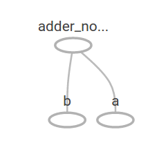
上面三个语句有点类似于 Python 中的 lambda 函数,对输入的变量(a 和 b)进行操作。通过向占位符传值来进行图的计算:
1 | print(sess.run(adder_node, {a: 3, b:4.5})) |
上述输出为:
1 | 7.5 |
在 TensorBoard 内,计算图如下:
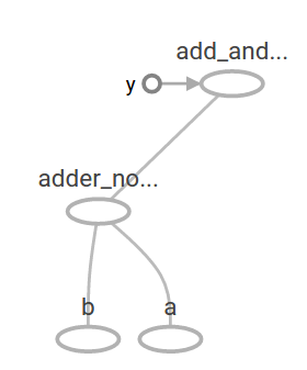
添加以下操作来得到更加复杂的计算图:
1 | add_and_triple = adder_node * 3. |
上述输出为:
1 | 22.5 |
在 TensorBoard 内,计算图如下所示:
在机器学习中,我们通常会想要一个可以接受任意输入的模型。为了使模型可训练,图形需要具有可修改性,使得在相同的输入下有新的输出。变量 Variable 允许我们向图中添加可训练的参数,具有类型和初始值:
1 | W = tf.Variable([.3], tf.float32) |
调用 tf.constant 时,常量被初始化,其中的值永远不会改变。相对地,调用 tf.Variable 时变量不会被初始化。要初始化 TensorFlow 程序中的所有变量,必须显式调用特殊的初始化方法,如下所示:
1 | init = tf.global_variables_initializer() |
init 是 TensorFlow 子图初始化所有的全局变量的句柄。这些变量在调用 sess.run 之后才会初始化。
由于 x 是占位符,我们可以同时对 linear_model 设置多个 x 的值,如下所示:
1 | print(sess.run(linear_model, {x:[1,2,3,4]})) |
输出为
1 | [ 0. 0.30000001 0.60000002 0.90000004] |
上面创建了一个模型,为了评估模型的表现,通过占位符 y 来提供所需的值,并且需要编写一个损失函数。
损失函数可以计算出当前模型与实际数据之间的偏差。我们将使用线性回归的标准损失模型,将当前模型与实际数据的差的平方相加。 创建一个向量 linear_model - y,其中每个元素都是对应的偏差量。我们先调用 tf.square 来计算偏差量的平方,然后通过 tf.reduce_sum 求和计算总的偏差:
1 | y = tf.placeholder(tf.float32) |
得到损失值为:
1 | 23.66 |
我们可以通过手动将 W 和 b 的值为设置为 -1 和 1,对模型进行改进。通过 tf.Variable 对变量进行初始化后,我们可以使用 tf.assign 等操作进行赋值。例如,W = -1 和 b = 1 是我们的模型的最优参数。我们可以按照如下语句设置 W 和 b :
1 | fixW = tf.assign(W, [-1.]) |
得到最优化输出:
1 | 0.0 |
我们可以通过手动设置猜测 W 和 b 的“完美”值,但机器学习的重点是可以自动设置正确的模型参数。下一节将展示如何完成此项工作。
tf.train API
本教程不对机器学习的过程进行介绍,建议先修相关知识。
TensorFlow 提供了优化器(optimizer),可以缓慢地更改每个变量,从而对损失函数进行最小化。最简单的优化器是梯度下降(gradient descent)。梯度下降根据变量的损失函数的导数,对每个变量进行修改。在 TensorFlow 中,优化器默认执行求导和反向传播等操作,如下所示:
1 | optimizer = tf.train.GradientDescentOptimizer(0.01) |
1 | sess.run(init) # reset values to incorrect defaults. |
得到最终的模型参数:
1 | [array([-0.9999969], dtype=float32), array([ 0.99999082], dtype=float32)] |
这里通过基本的 TensorFlow 核心代码完成了最简单的机器学习。如需将复杂的模型和方法将数据输入到自己的计算模型中,则需要更多的代码。因此,TensorFlow 对常见的模式、结构和函数提供了更高级别的抽象。我们将在下一节中学习如何使用其中的一些抽象。
完整程序
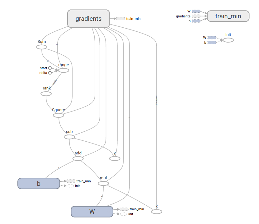
完整的可训练线性回归模型如下所示:
1 | import numpy as np |
运行后输出
1 | W: [-0.9999969] b: [ 0.99999082] loss: 5.69997e-11 |
这个更复杂的程序仍然可以在 TensorBoard 中可视化:
tf.estimator
tf.estimator 是一个高级 TensorFlow 库,简化了机器学习的机制,包括:
- 运行训练循环
- 运行评估循环
- 管理数据集
tf.estimator 定义了许多常见的模型。
基本用法
tf.estimator 可以高度简化线性回归程序:
1 | # NumPy is often used to load, manipulate and preprocess data. |
运行后输出:
1 | train metrics: {'average_loss': 1.4833182e-08, 'global_step': 1000, 'loss': 5.9332727e-08} |
虽然评估数据集具有相对更高的损失,但这个损失仍然接近于零,意味着学习过程有效。
自定义模型
tf.estimator 不要求使用其预定义的模型。我们可以创建自定义模型,同时仍然可以保持 tf.estimator 的数据集合,反馈,训练等的高级抽象。下面将展示如何通过低级 TensorFlow API 来实现具有相同功能的 LinearRegressor 模型。
要定义一个能够通过 tf.estimator 工作的自定义模型,需要使用 tf.estimator.Estimator。上节中的 tf.estimator.LinearRegressor 实际上是 tf.estimator.Estimator 的一个子类。为了实现相同功能,我们只需要提供一个函数 model_fn 来告诉 tf.estimator 如何计算预测结果,训练步骤和损失。代码如下:
1 | import numpy as np |
运行时输出:
1 | train metrics: {'loss': 1.227995e-11, 'global_step': 1000} |
可以看到,自定义函数 model_fn() 与之前的 API 章节的手动循环训练过程非常类似。