ROC 和 AUC

在信号检测理论中,接收者操作特征(Receiver Operating Characteristic,ROC)曲线是是一种坐标图式的分析工具,通过计算 ROC 的曲线下面积(Area Under Curve,AUC)可以对分类模型进行评估。

ROC 分析的是二分分类模型。

ROC 曲线是通过绘制采用不同分类阈值时的 TPR 与 FPR 来选择模型。ROC 曲线的对角线可以被解释为随机猜测(如丢硬币、正反面出现概率预测均是 50%),并且落在对角线上方的分类模型优于随机猜测,落在对角线下方的分类模型比随机猜测更差。完美的分类器将落入图的左上角,TPR 为 1,FPR 为 0。降低分类阈值会导致将更多样本归为正类别,从而增加假正例和真正例的个数。

下文将实现分类器的 ROC 曲线绘制,该分类器仅使用 wdbc 数据集中的两个特征来预测肿瘤是良性还是恶性。

数据导入和预处理

1
2
3
4
5
6
7
8
9
10
11
12
13
14
15
16
17
18
import pandas as pd
import numpy as np
import matplotlib.pyplot as plt
from sklearn.model_selection import StratifiedKFold
from sklearn.preprocessing import LabelEncoder
from sklearn.model_selection import train_test_split
from sklearn.preprocessing import StandardScaler
from sklearn.decomposition import PCA
from sklearn.linear_model import LogisticRegression
from sklearn.pipeline import make_pipeline

df = pd.read_csv('https://archive.ics.uci.edu/ml/machine-learning-databases/breast-cancer-wisconsin/wdbc.data',
header=None)
X = df.loc[:, 2:].values
y = df.loc[:, 1].values
le = LabelEncoder()
y = le.fit_transform(y)
X_train, X_test, y_train, y_test = train_test_split(X, y, test_size=0.20, stratify=y, random_state=1)

ROC 曲线的 scikit-learn 实现

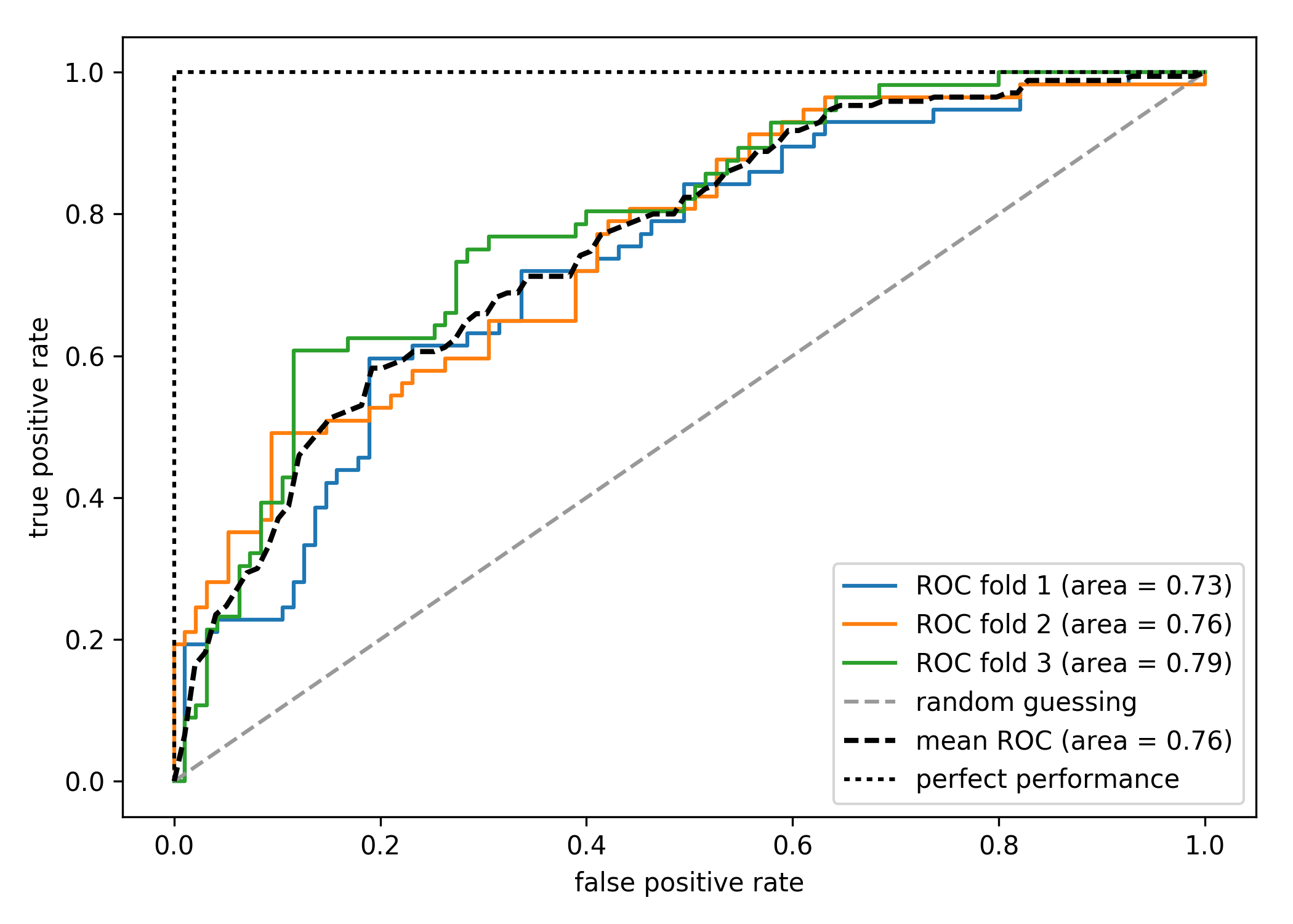
使用逻辑回归 pipeline,并采用折叠数为 3 的 StratifiedKFold,如下代码:

1
2
3
4
5
6
7
8
9
10
11
12
13
14
15
16
17
18
19
20
21
22
23
24
25
26
27
28
29
30
from sklearn.metrics import roc_curve, auc
from scipy import interp

pipe_lr = make_pipeline(StandardScaler(),
PCA(n_components=2),
LogisticRegression(penalty='l2', random_state=1, C=100.0))

X_train2 = X_train[:, [4, 14]]
cv = list(StratifiedKFold(n_splits=3, random_state=1).split(X_train, y_train))

fig = plt.figure(figsize=(7, 5))

mean_tpr = 0.0
mean_fpr = np.linspace(0, 1, 100)
all_tpr = []

for i, (train, test) in enumerate(cv):
probas = pipe_lr.fit(X_train2[train], y_train[train]).predict_proba(X_train2[test])
fpr, tpr, thresholds = roc_curve(y_train[test], probas[:, 1], pos_label=1)
mean_tpr += interp(mean_fpr, fpr, tpr)
mean_tpr[0] = 0.0
roc_auc = auc(fpr, tpr)
plt.plot(fpr, tpr, label='ROC fold {} (area = {:.2f}'.format(i + 1, roc_auc))

plt.plot([0, 1], [0, 1], linestyle='--', color=(0.6, 0.6, 0.6), label='random guessing')

mean_tpr /= len(cv)
mean_tpr[-1] = 1.0
mean_auc = auc(mean_fpr, mean_tpr)
plt.plot(mean_fpr, mean_tpr, 'k--', label='mean ROC (area = {:.2f}'.format(mean_auc), lw=2)

上面的代码通过从 SciPy 导入的 interp 函数插入了三次折叠的平均 ROC 曲线,并通过 auc 函数计算曲线下面积。

三次绘制的 ROC 曲线表明不同折叠之间存在一定程度的变化,并且 ROC AUC 的平均值 (0.76) 落在完美预测 (1.0) 和随机猜测 (0.5) 之间:

如果只需要用到 ROC AUC 分数,也可以直接导入 sklearn.metrics.roc_auc_score 函数。ROC AUC 分数可以对样本数量不平均的二分分类模型进行评估。