逻辑回归(Logistic Regression)是一种非常容易实现的分类模型,对于线性可分的情况有很好的表现。
与之前文章中的感知器和 Adaline 类似,本文中的逻辑回归也是二元分类的线性模型。
算法思想
为了解释逻辑回归模型背后的思想,先介绍一个概念:比值比(Odds ratio, OR)。
比值比的数学表示为 $\cfrac p {1-p}$,其中 $p$ 为某事件可能发生的几率。
在此基础上,定义 logit 函数,即比值比的对数(计算机科学中 $\log$ 表示自然对数):
logit 的作用是将范围为 $(0,1)$ 的变量,映射到整个实数集。
对于给定的 $x$:
- $y=1$ 的概率 $p(y=1\ | x)$ 在 $(0,1)$ 之间。
- 基于神经元模型,输出的概率是由净输入 $z = \sum_{i=0}^m w_i x_i = w^T x$ 得到的。
基于以上逻辑,建立 $p(y=1\ \mid x) \rightarrow z$ 的 logit 映射:
因此,logit 的反函数即为 $z \rightarrow p(y=1\ \mid x)$ 的映射:
这里 $\phi (z) = \cfrac 1 {1+e^{-z}}$ 称为 logistic sigmoid 函数,通常简称为 sigmoid 函数。(sigmoid 意为 S-shaped,即 S 形状的曲线。)
1 | import matplotlib.pyplot as plt |

算法模型
Adaline 和 逻辑回归的差异,如下图所示:

Adaline:
- 激活函数:线性函数 $\phi (z) = z$
- 阈值函数:阶跃函数 $\hat y = \begin{cases} 1 & if \ \phi (z) \ge 0 \\[2ex] 0 & otherwise \end{cases}$
逻辑回归:
- 激活函数:sigmoid 函数 $\phi (z) = \cfrac 1 {1+e^{-z}}$
- 阈值函数:阶跃函数 $\hat y = \begin{cases} 1 & if \ \phi (z) \ge 0.5 \\[2ex] 0 & otherwise \end{cases}$
需要注意的是,逻辑回归中的条件 $\phi (z) \ge 0.5$,等价于 $z \ge 0$。
损失函数和成本函数
定义损失函数(Loss Fucntion)和成本函数(Cost Fucntion),以训练权重参数 $w$。
损失函数用于单个样本,代表预测输出 $\hat y^{(i)}$ 和实际输出 $y^{(i)}$ 之间的误差。
$$\begin{align} L(\hat y^{(i)}, y^{(i)}) & = -[y^{(i)} \log (\hat y^{(i)}) + (1 - y^{(i)}) \log (1 - \hat y^{(i)})] \\ & = \begin{cases} -\log (\hat y^{(i)}) & \text{if} \ y^{(i)} = 1 \\[2ex] -\log (1 - \hat y^{(i)}) & \text{if} \ y^{(i)} = 0\end{cases} \end{align}$$- 当 $y^{(i)} = 1$ 时,最小化 $L$ 等价于 $\hat y^{(i)}$ 接近于 1。
- 当 $y^{(i)} = 0$ 时,最小化 $L$ 等价于 $\hat y^{(i)}$ 接近于 0。
成本函数是整个训练集的损失函数的平均值。最小化成本函数,可以得到最优的参数 $w$。
$$\begin{align} J(w) & = {\frac 1 m} \sum _{i=1}^m L(\hat y^{(i)}, y^{(i)}) \\ & = -{\frac 1 m} \sum _{i=1}^m [y^{(i)} \log (\hat y^{(i)}) + (1 - y^{(i)}) \log (1 - \hat y^{(i)})] \end{align}$$Python 实现
逻辑回归的实现如下,使用梯度下降法进行参数训练:
1 | import numpy as np |
绘制图像
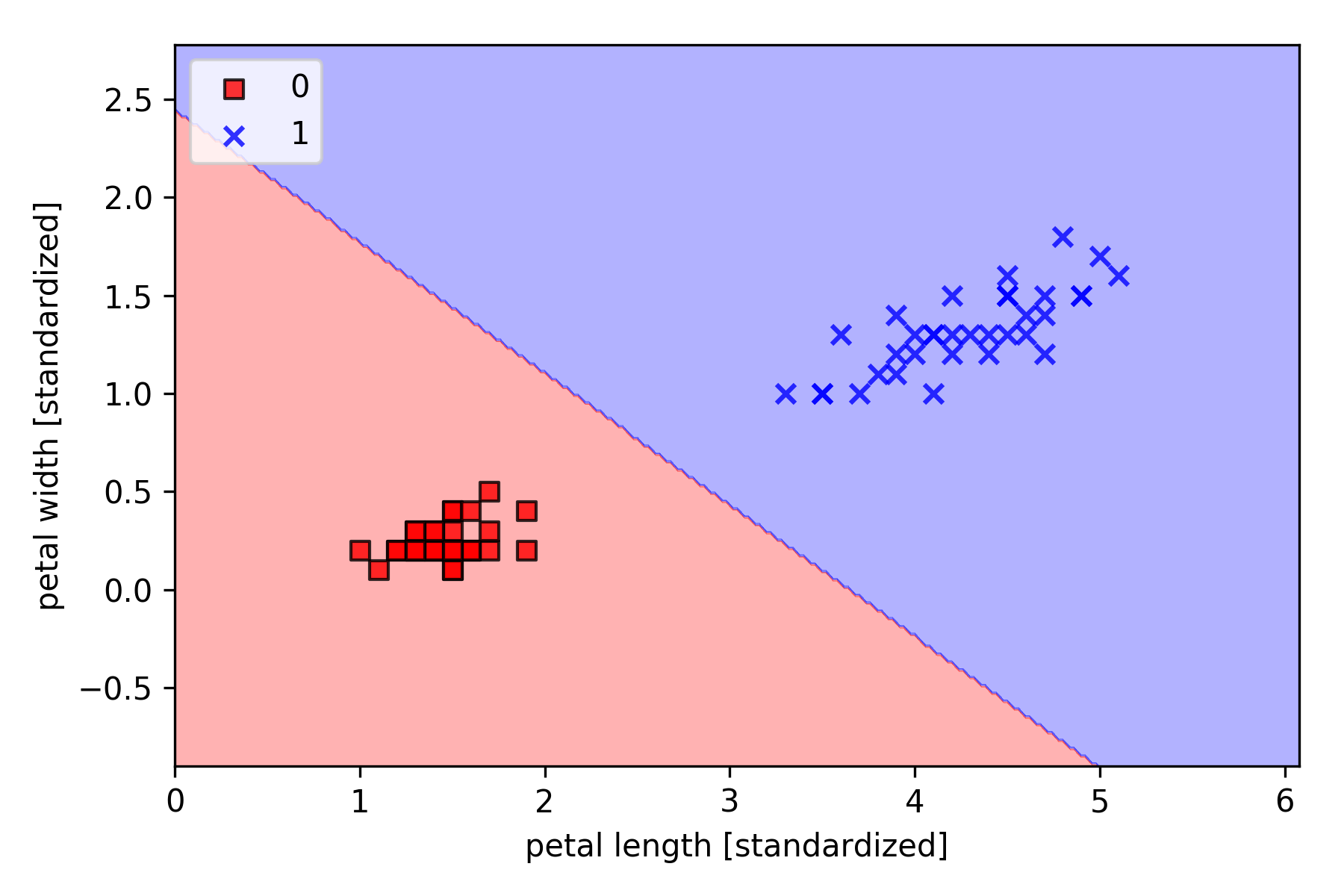
以 Iris-setosa(标签 0) and Iris-versicolor(标签 1)为例,采用逻辑回归分类,绘制决策边界如下,
1 | import matplotlib.pyplot as plt |